Code
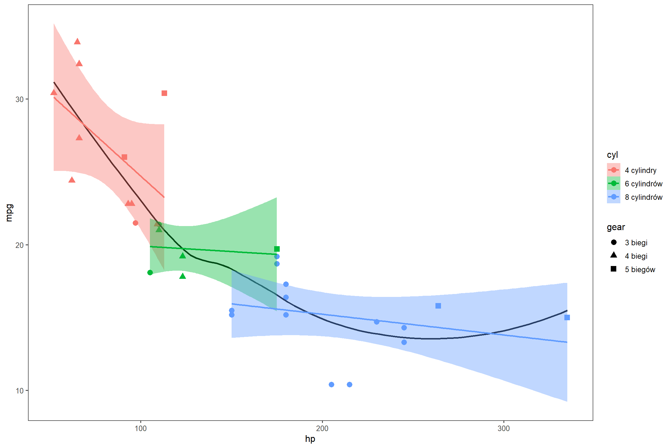
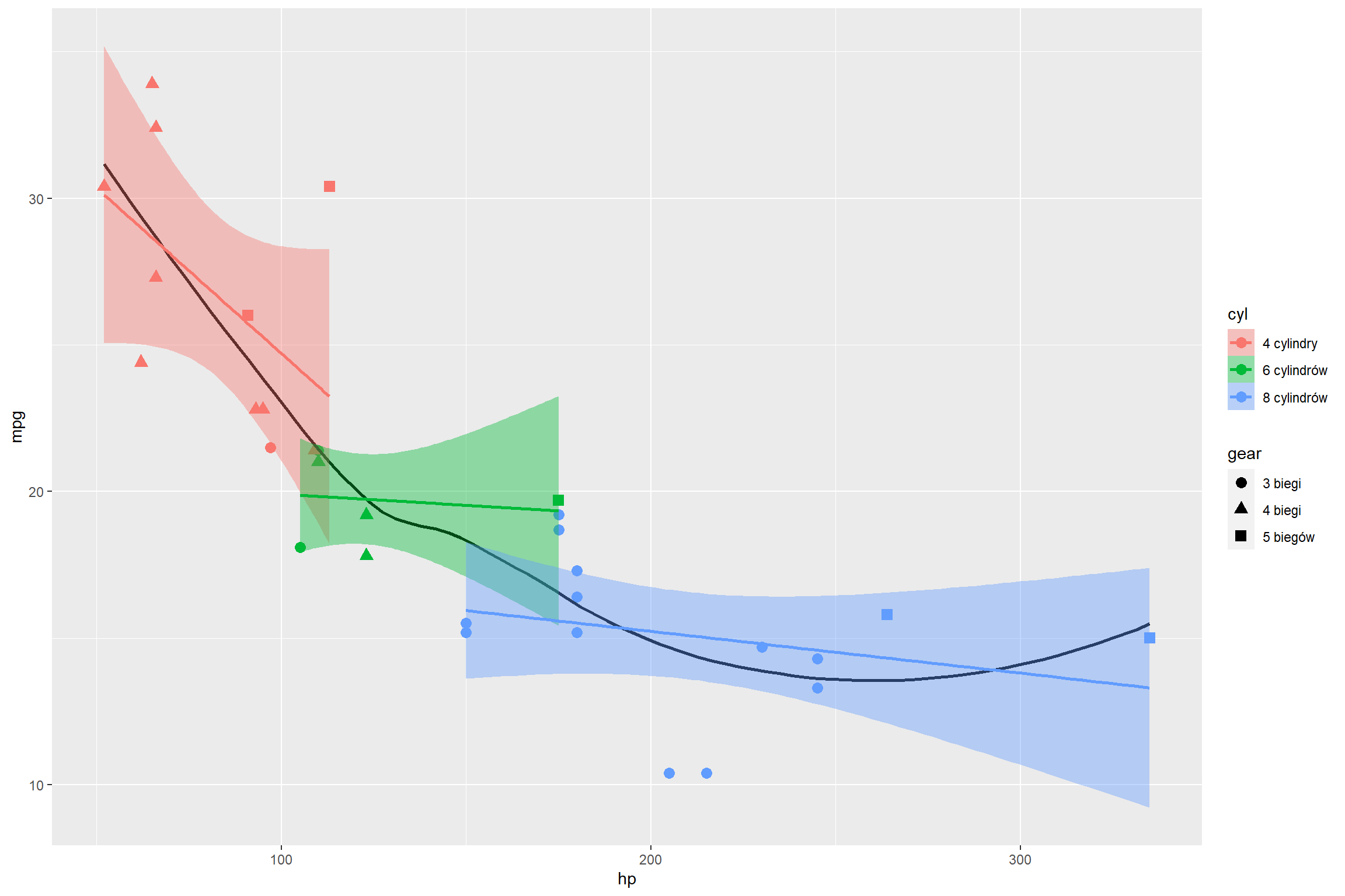
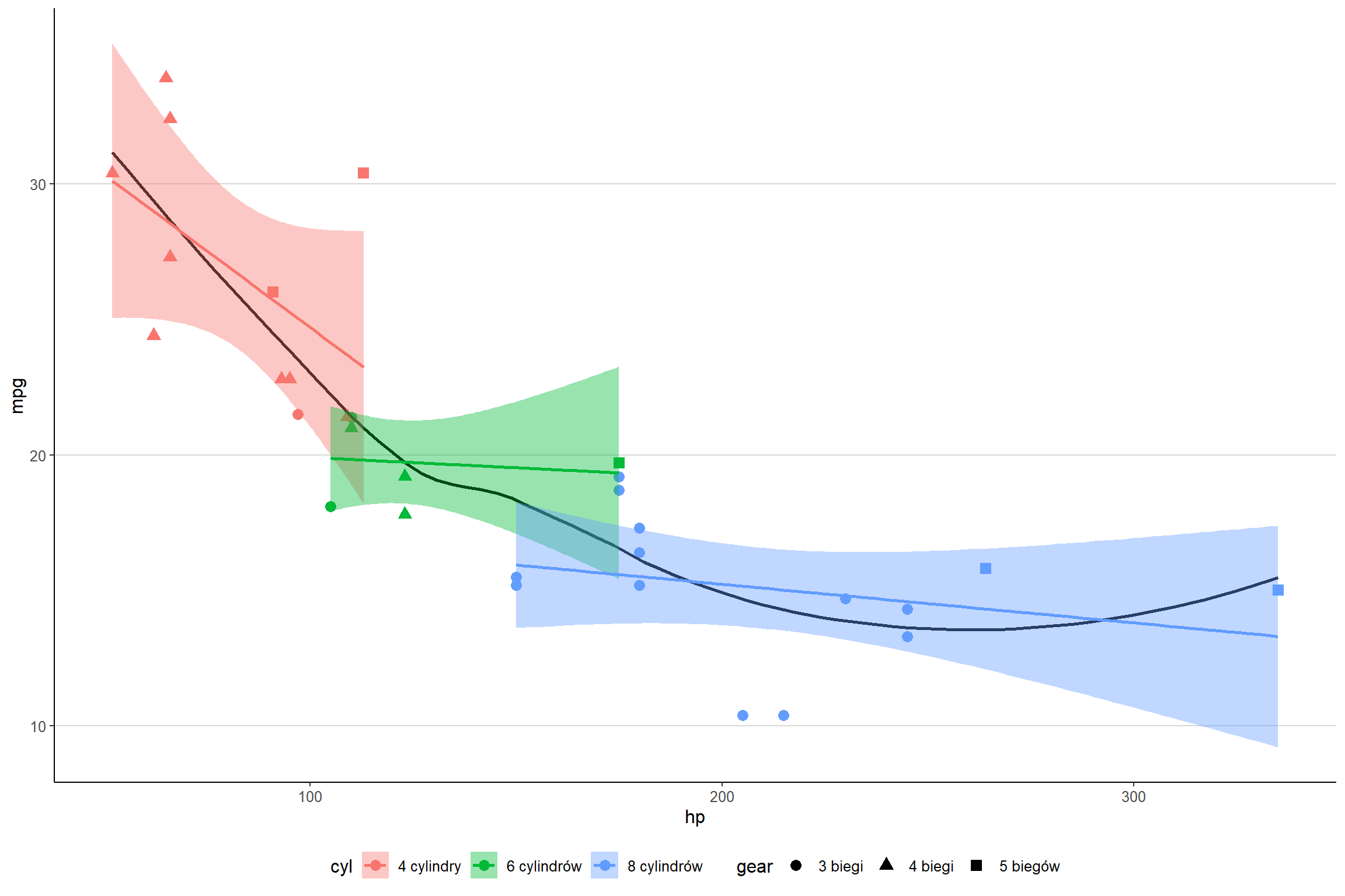
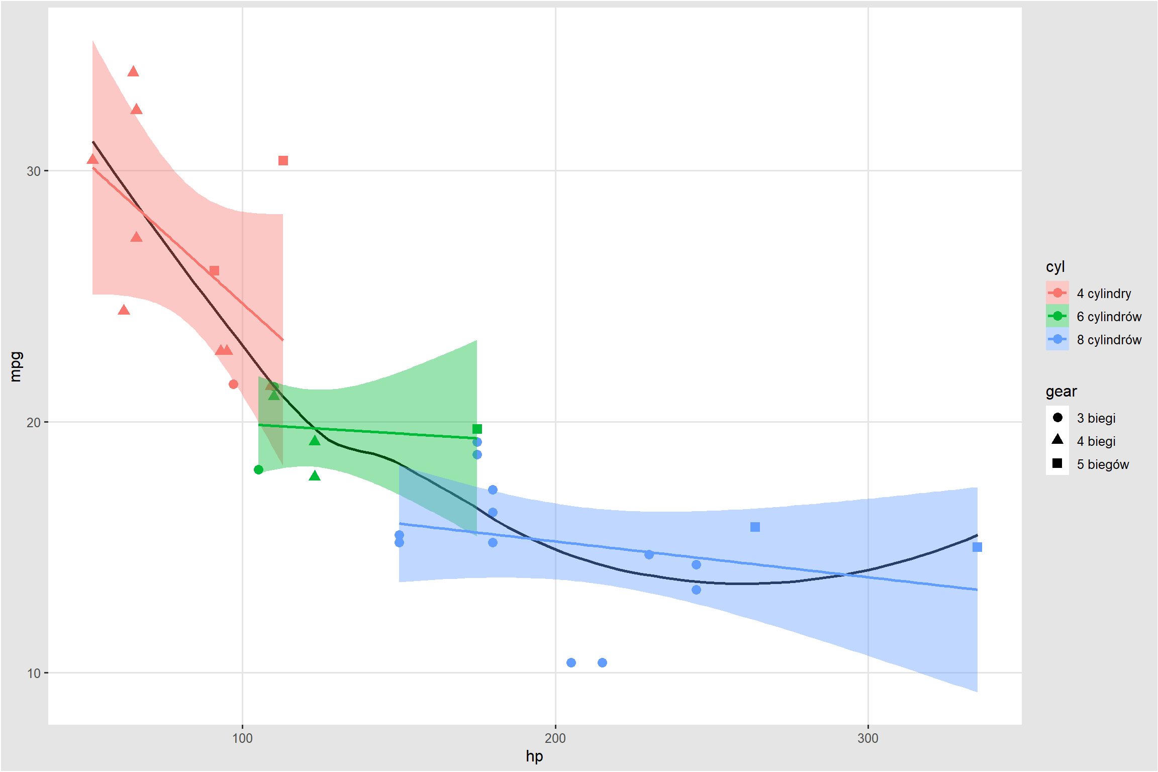
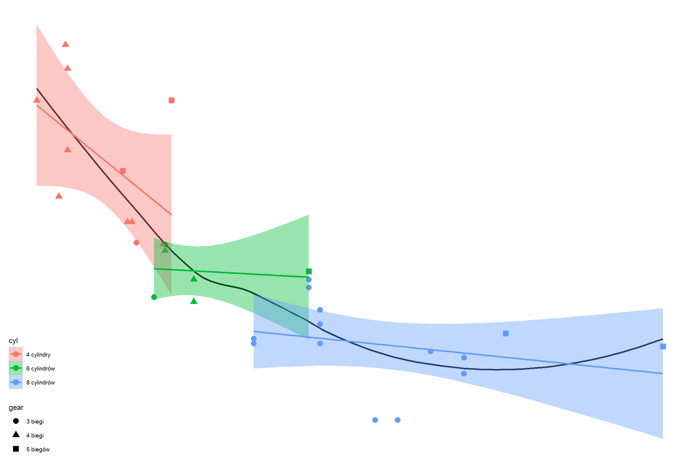
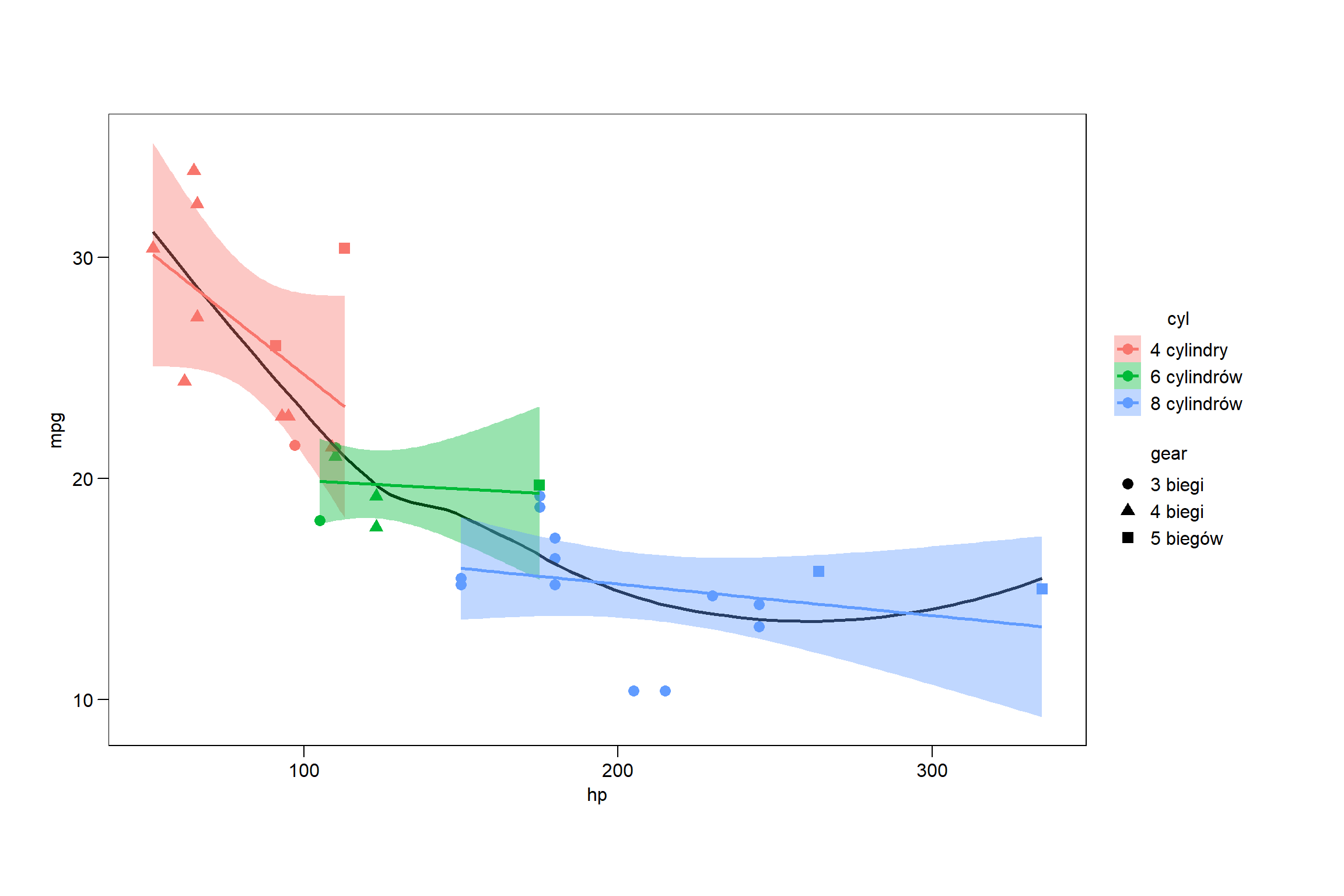
library(ggplot2)
library(ggthemes)
data(mtcars)
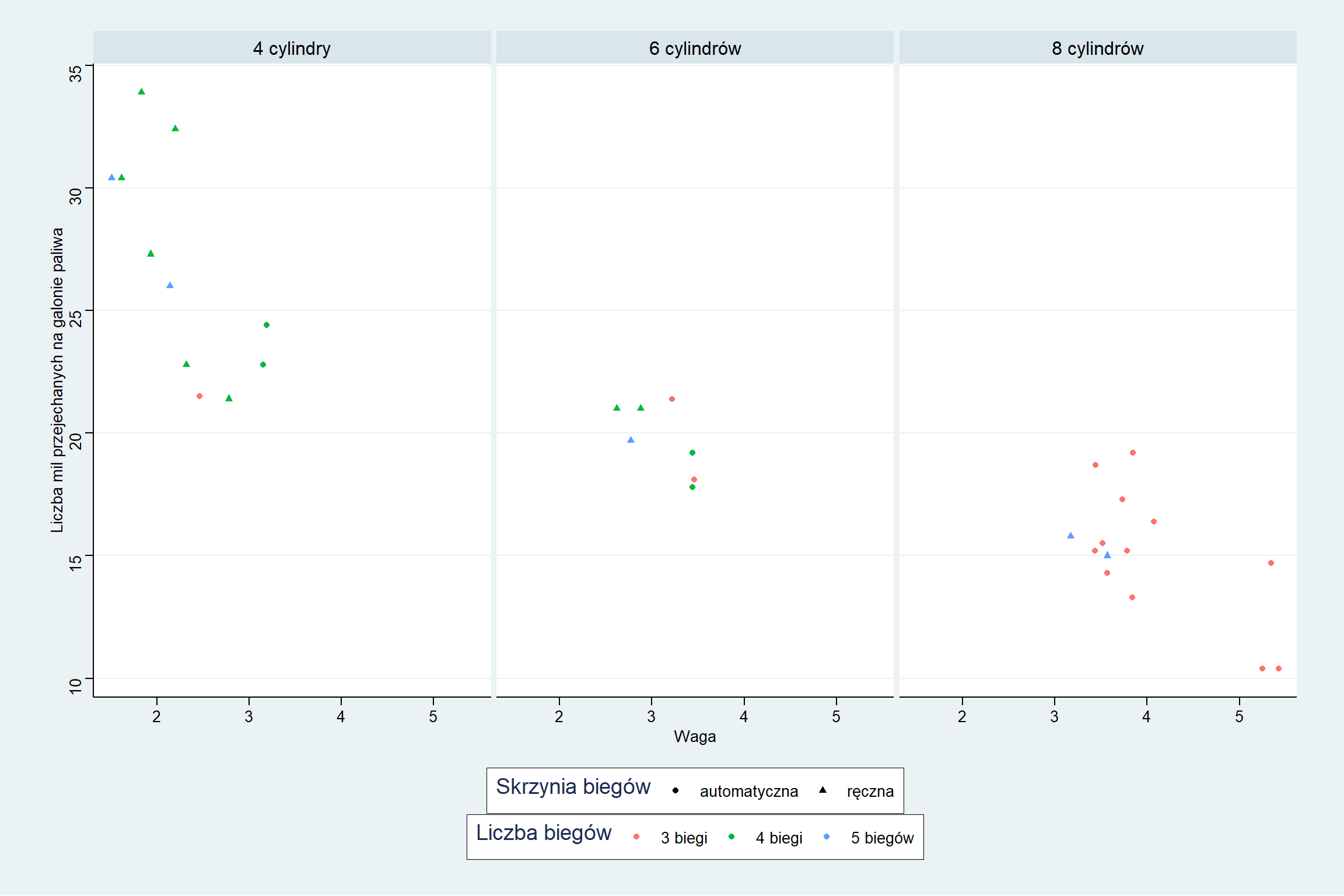
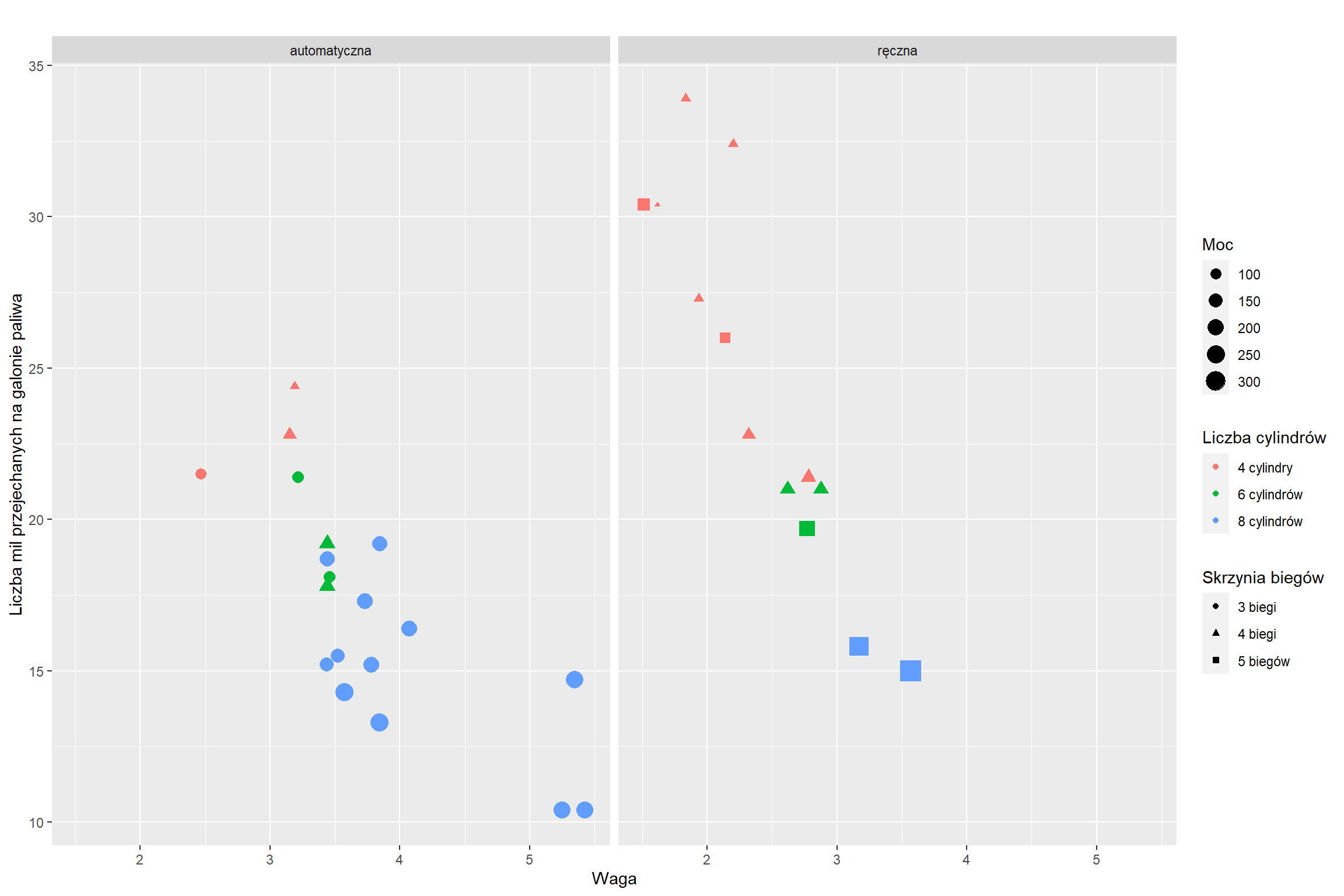
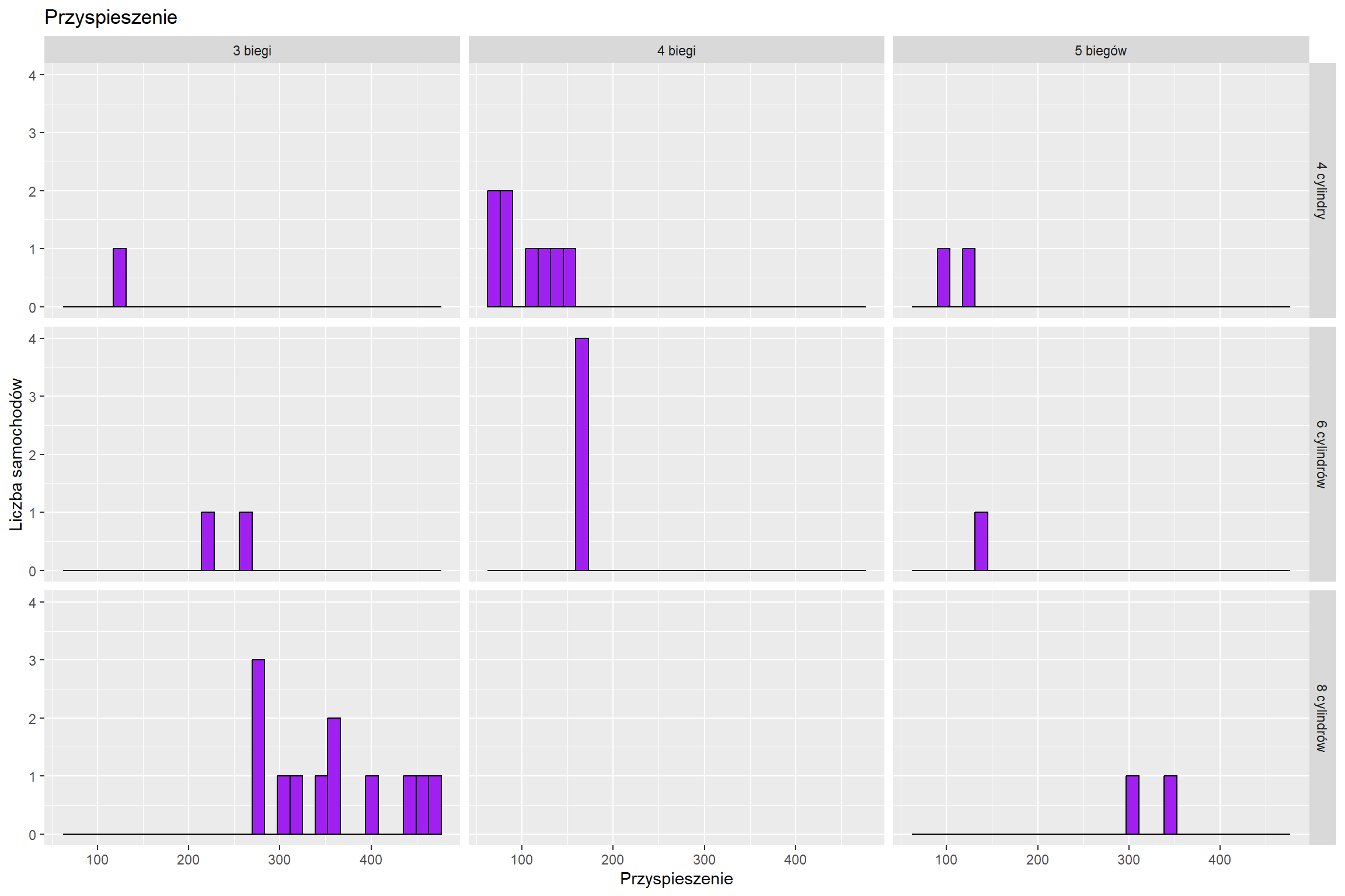
mtcars$gear <- factor(mtcars$gear,levels=c(3,4,5),labels=c('3 biegi', '4 biegi', '5 biegów'))
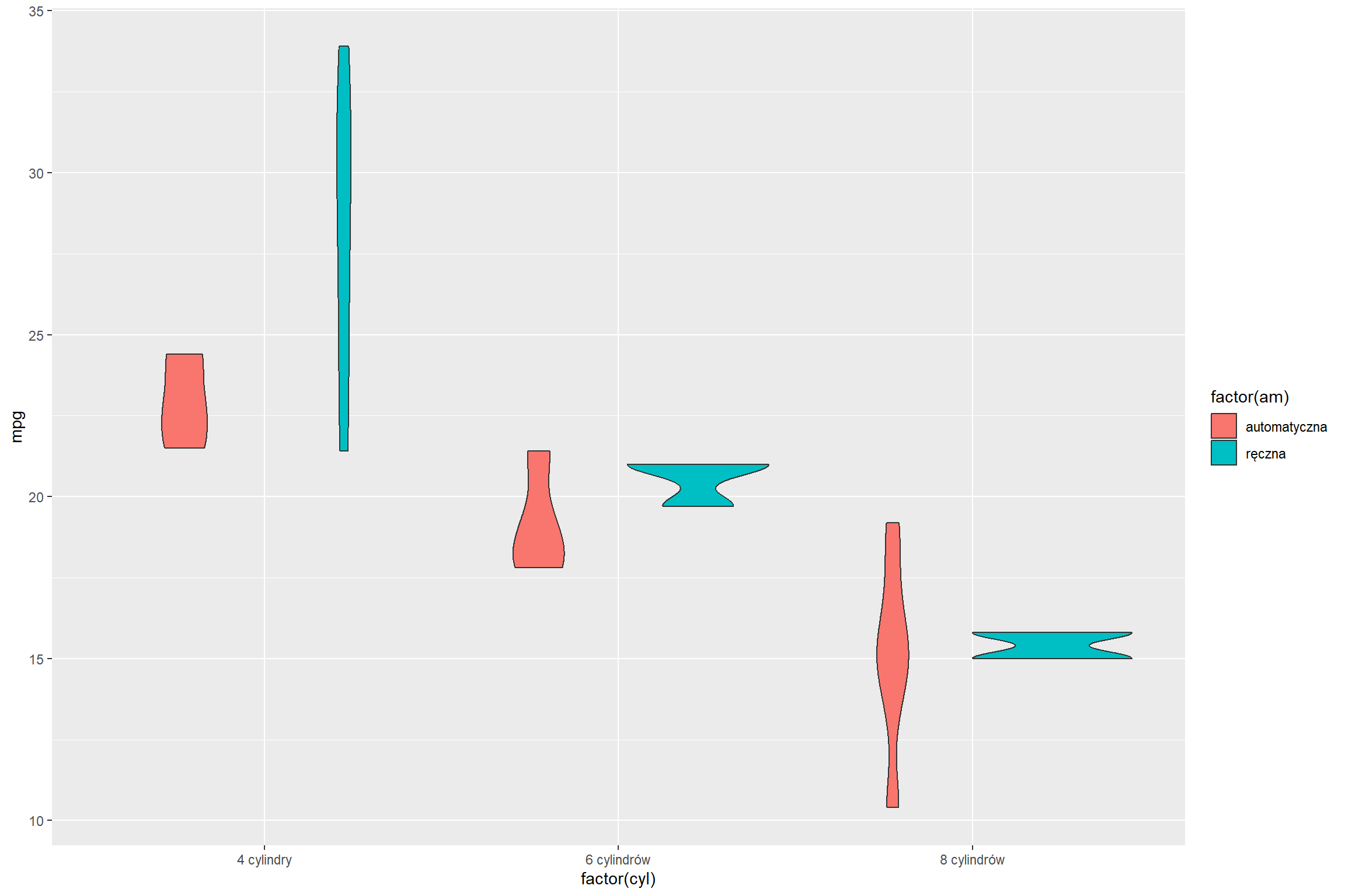
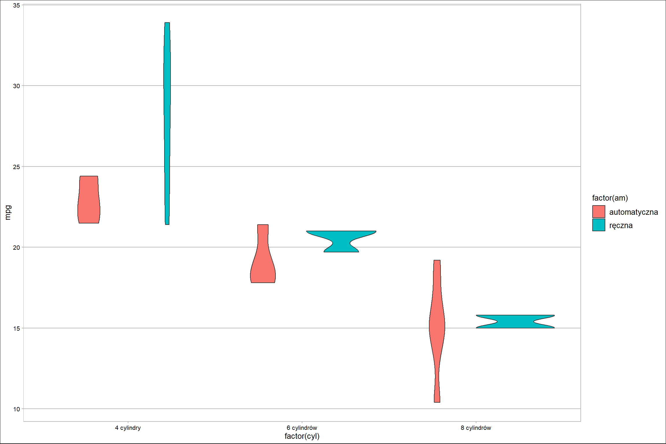
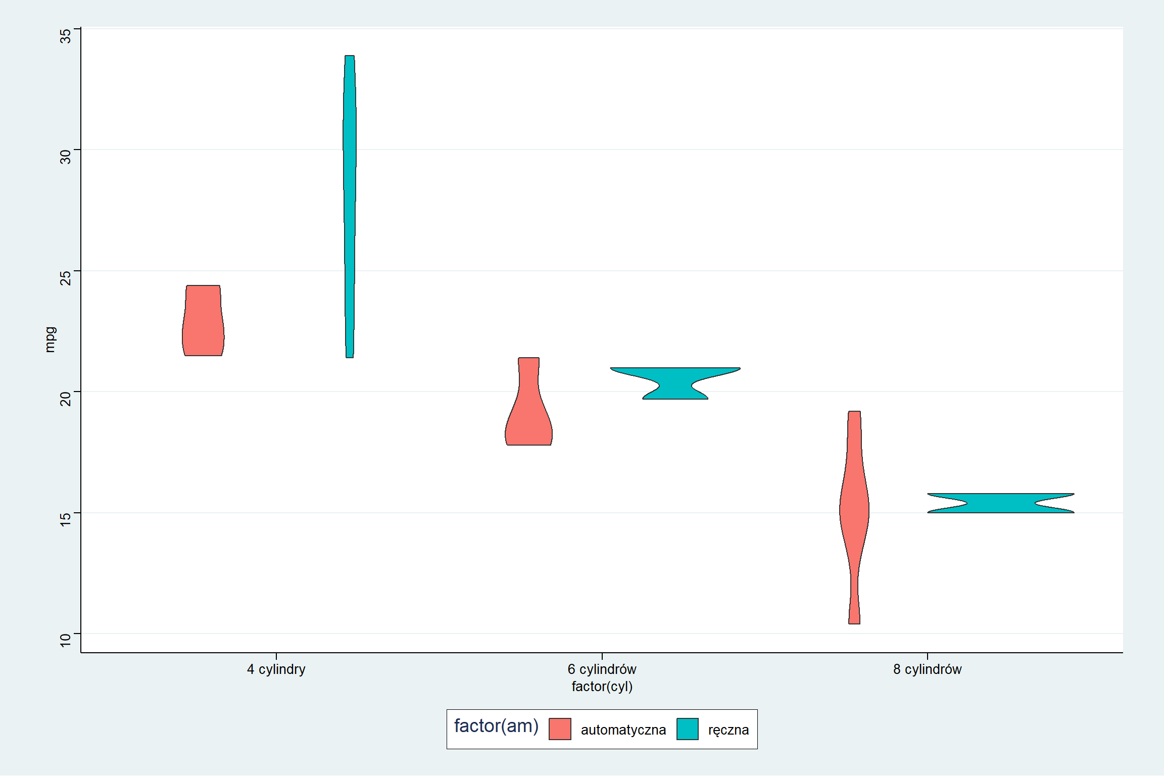
mtcars$am <- factor(mtcars$am, levels = c(0,1), labels = c('automatyczna','ręczna'))
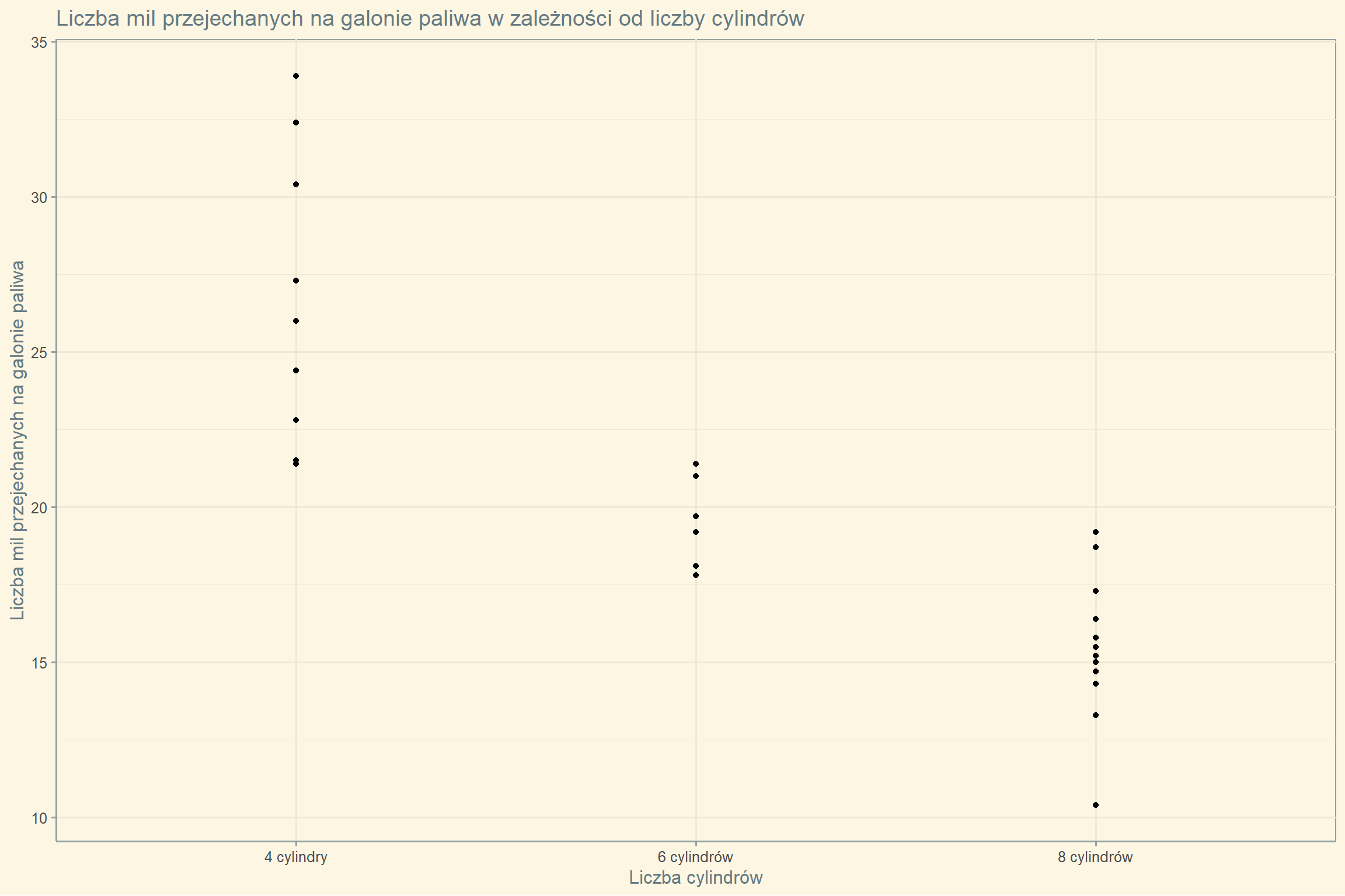
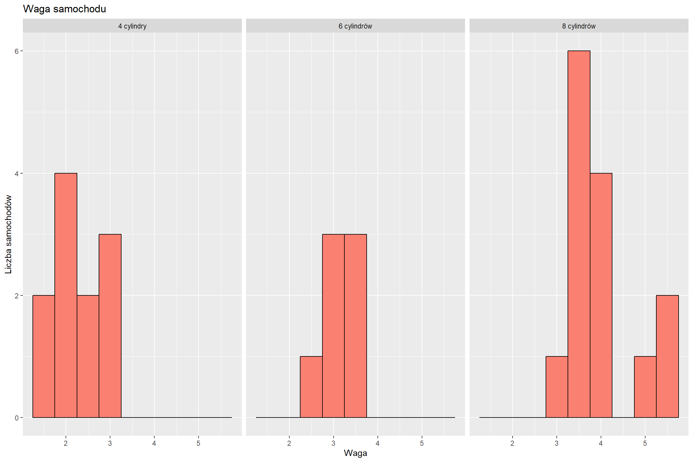
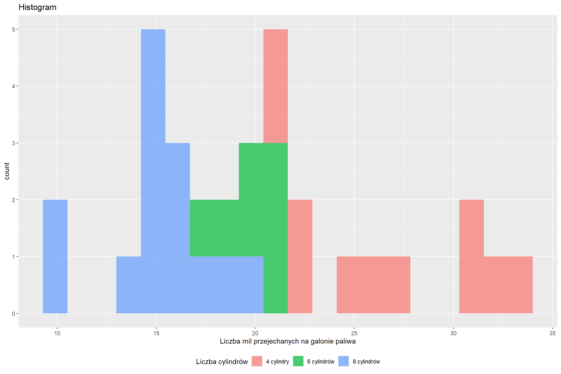
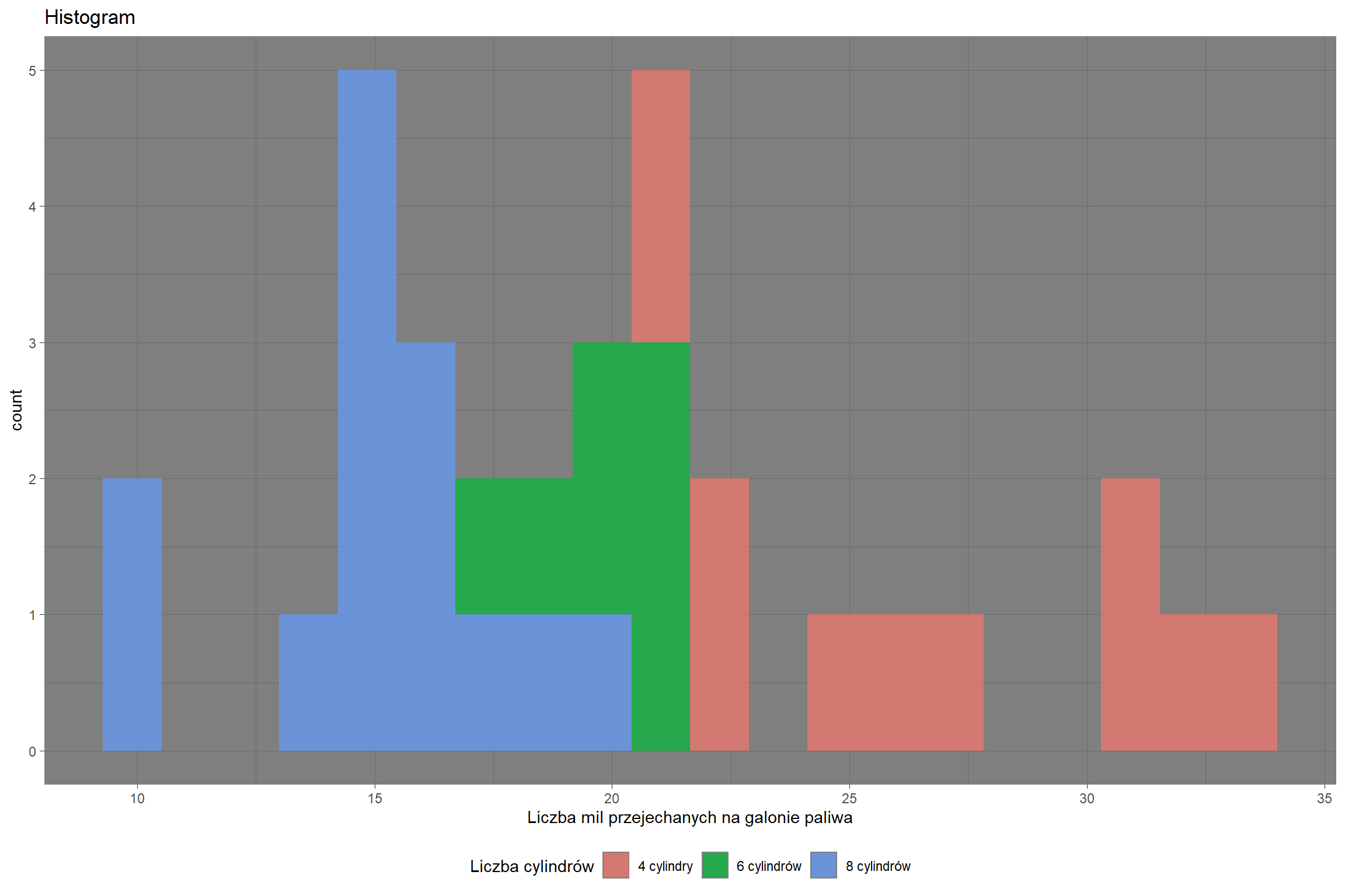
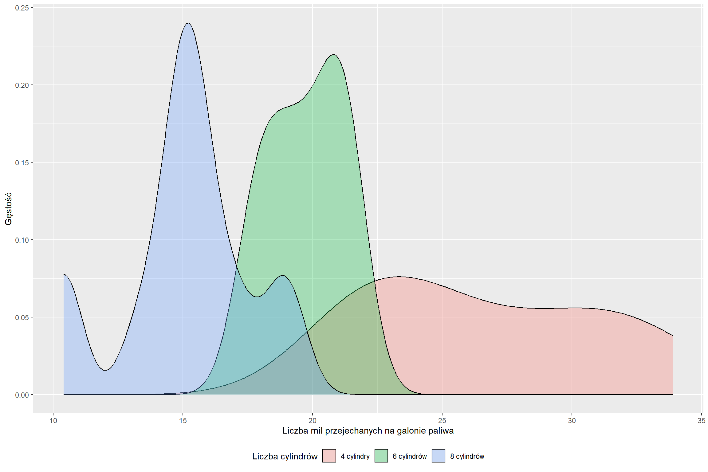
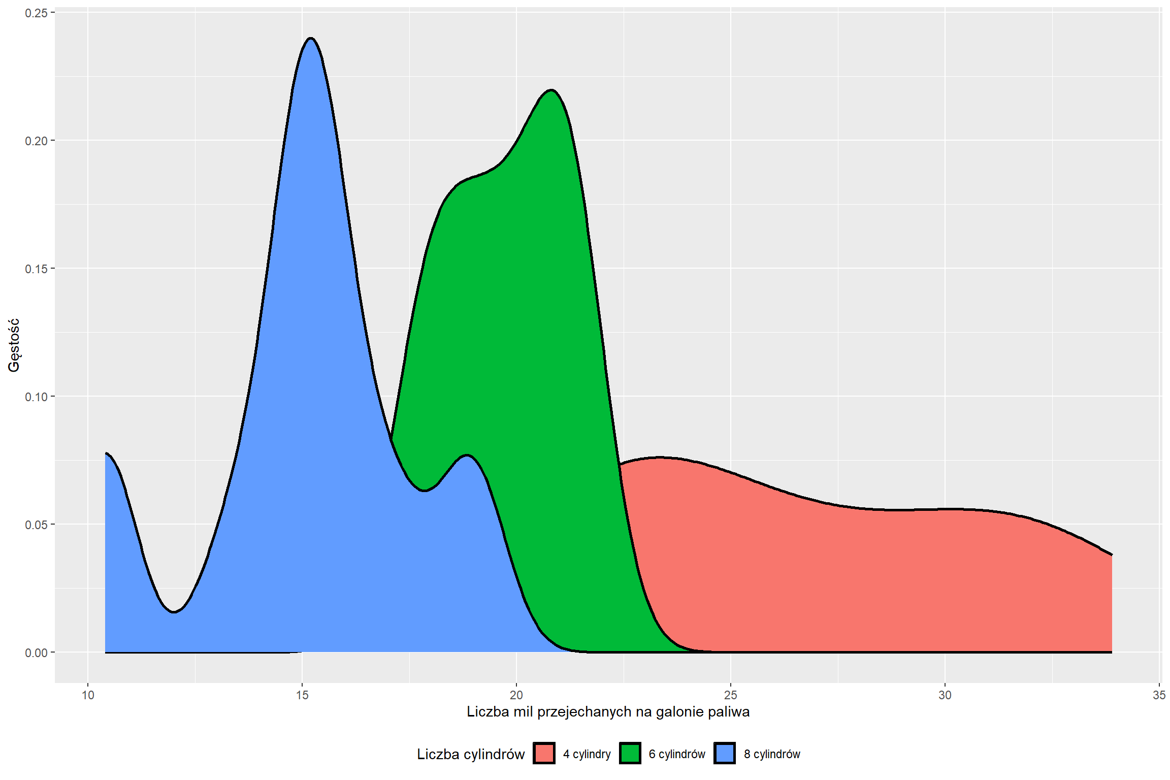
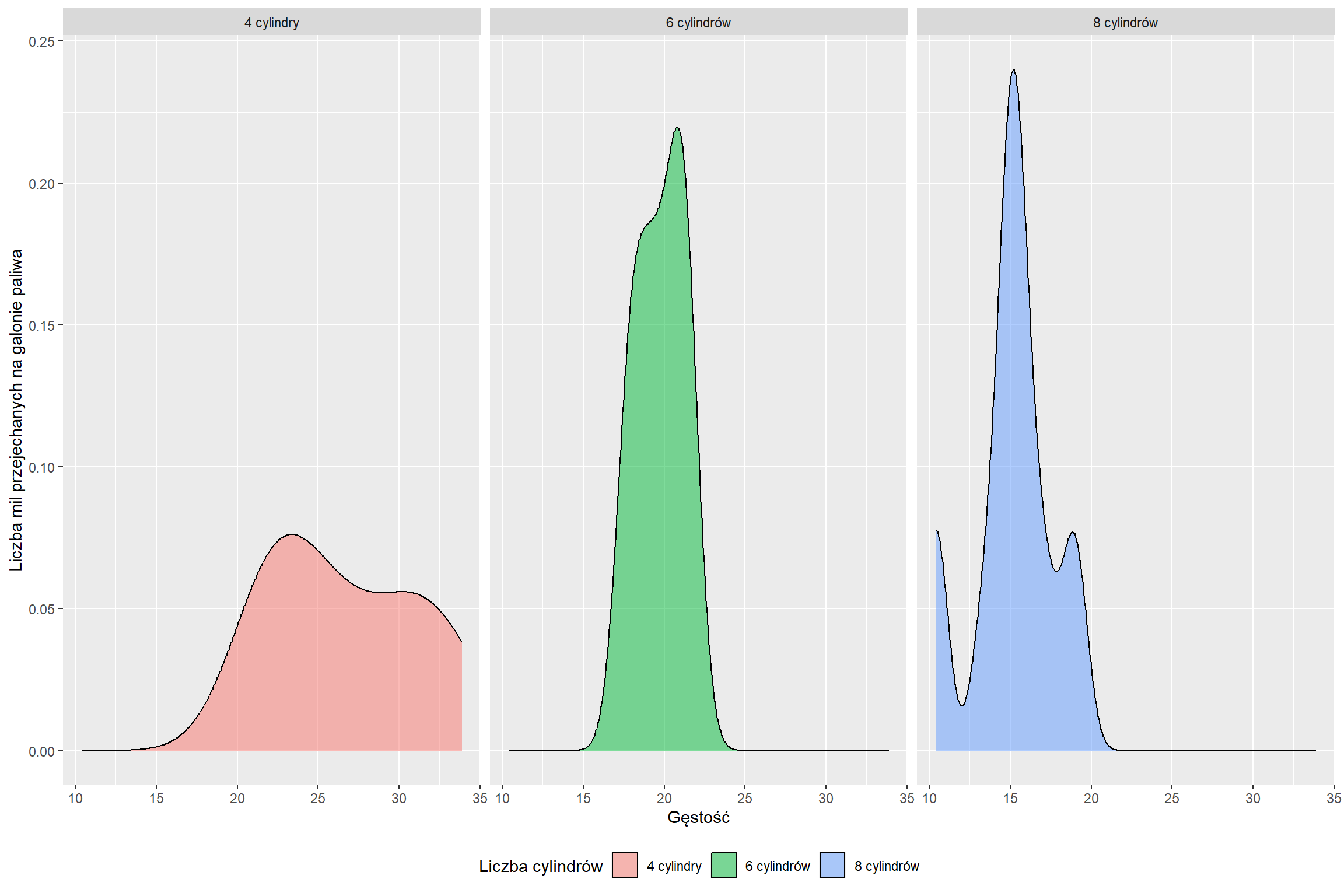
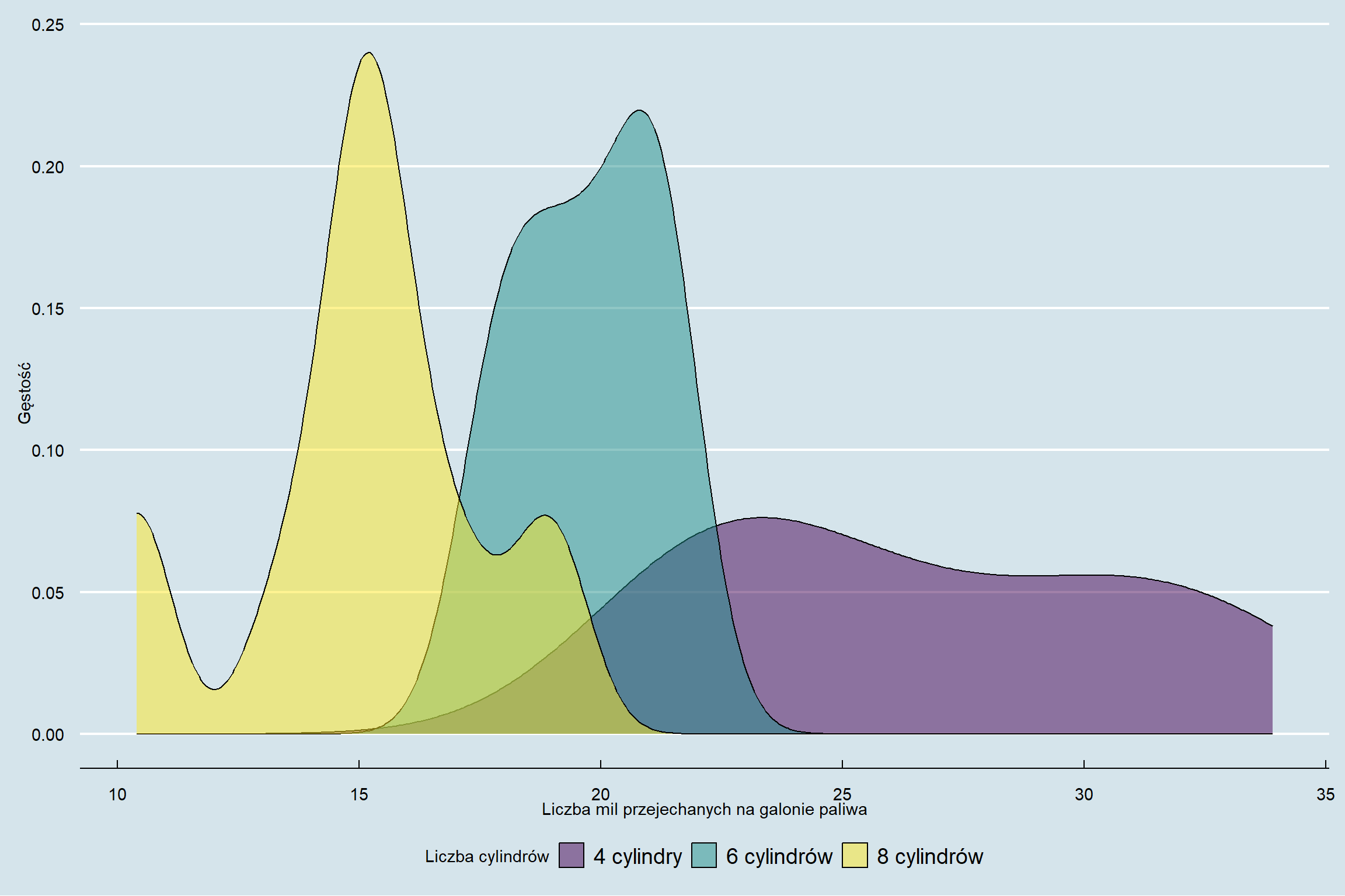
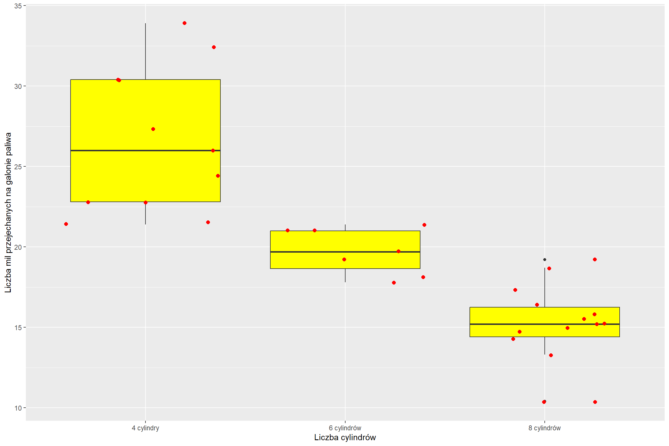
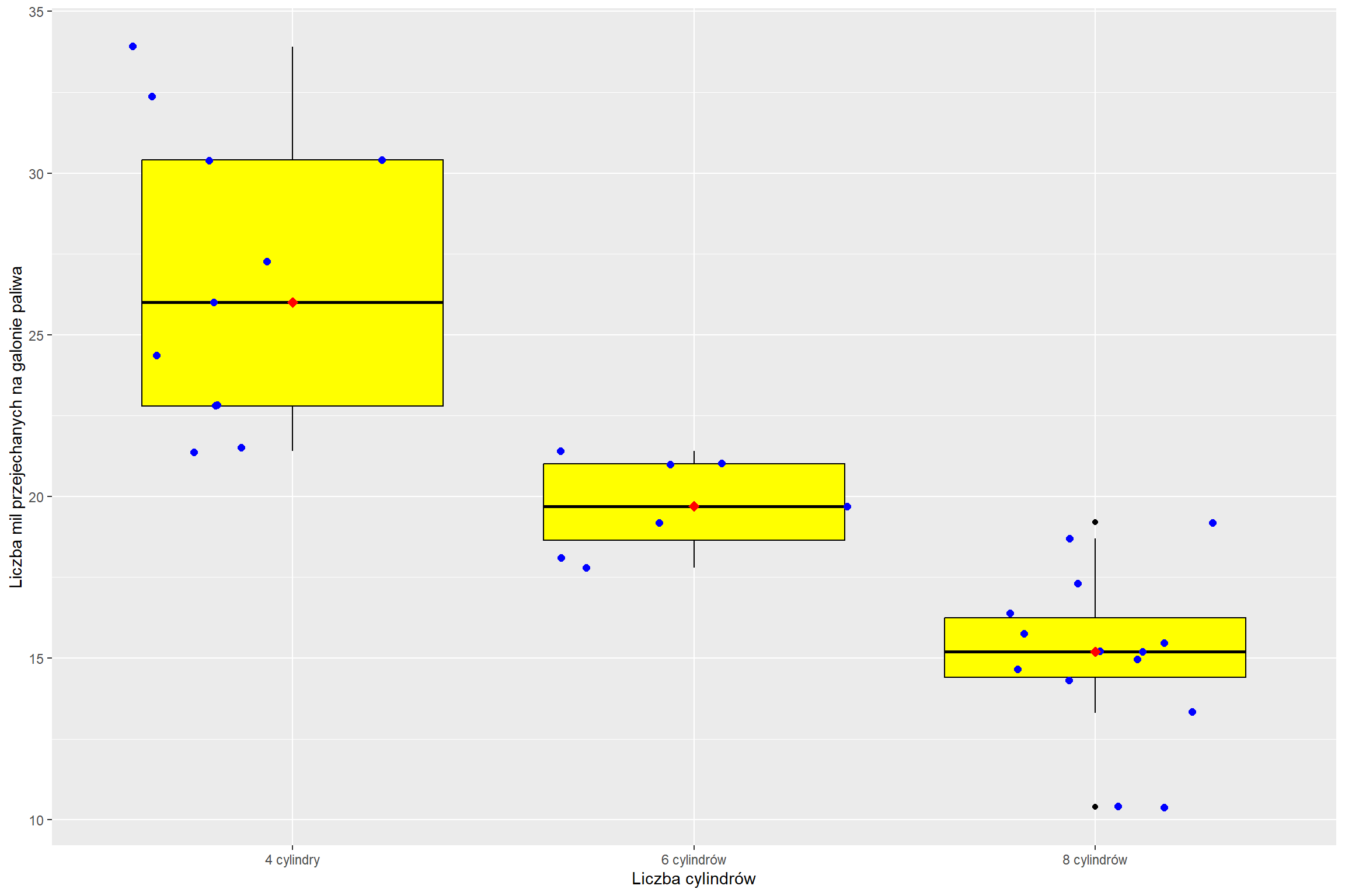
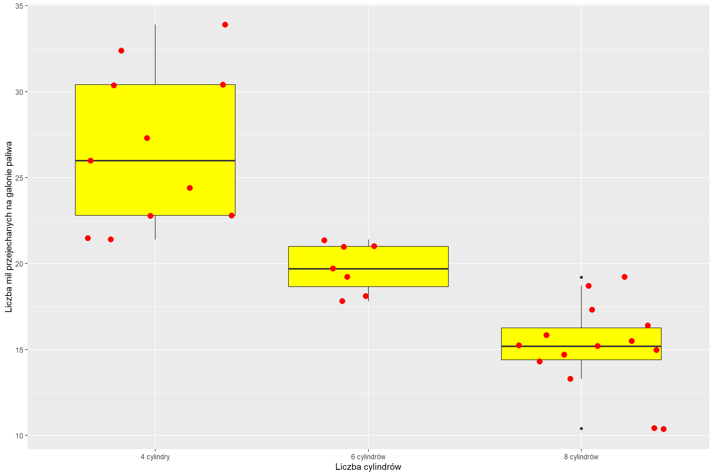
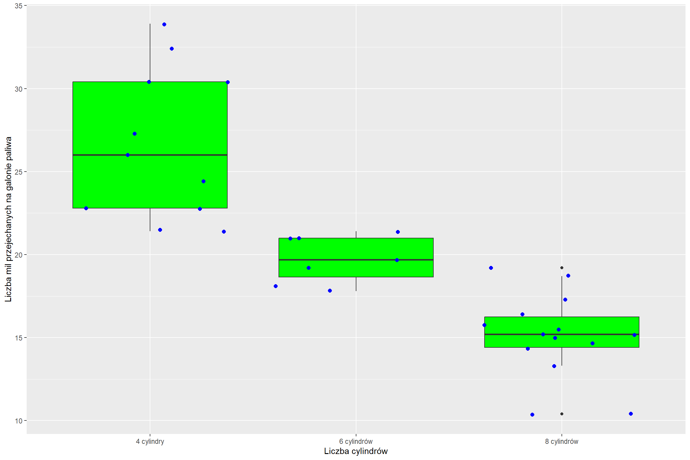
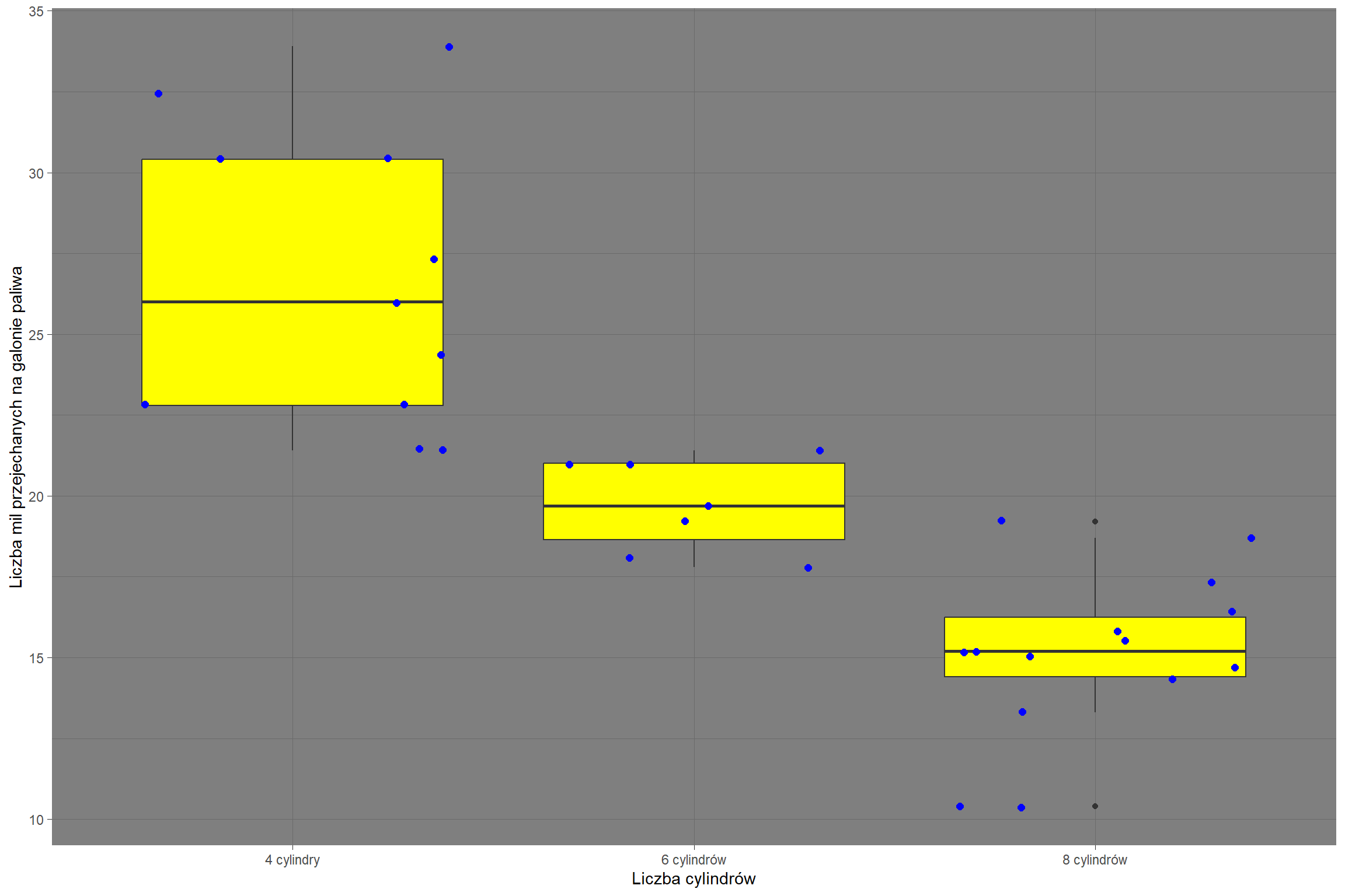
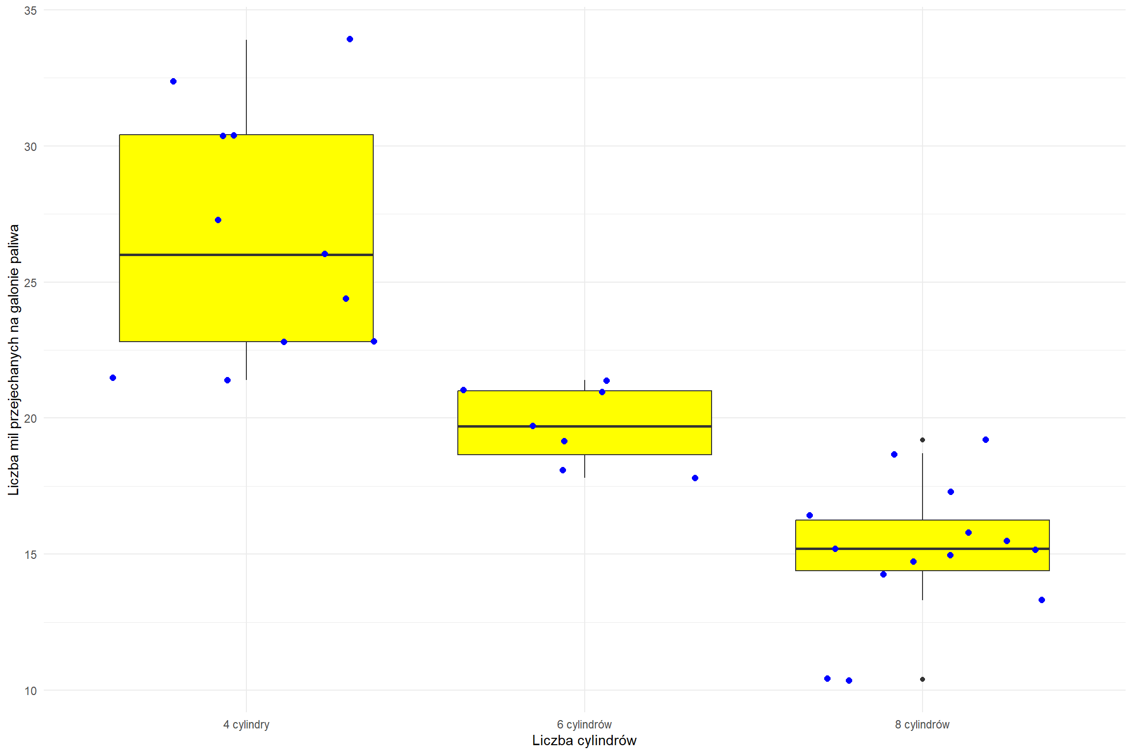
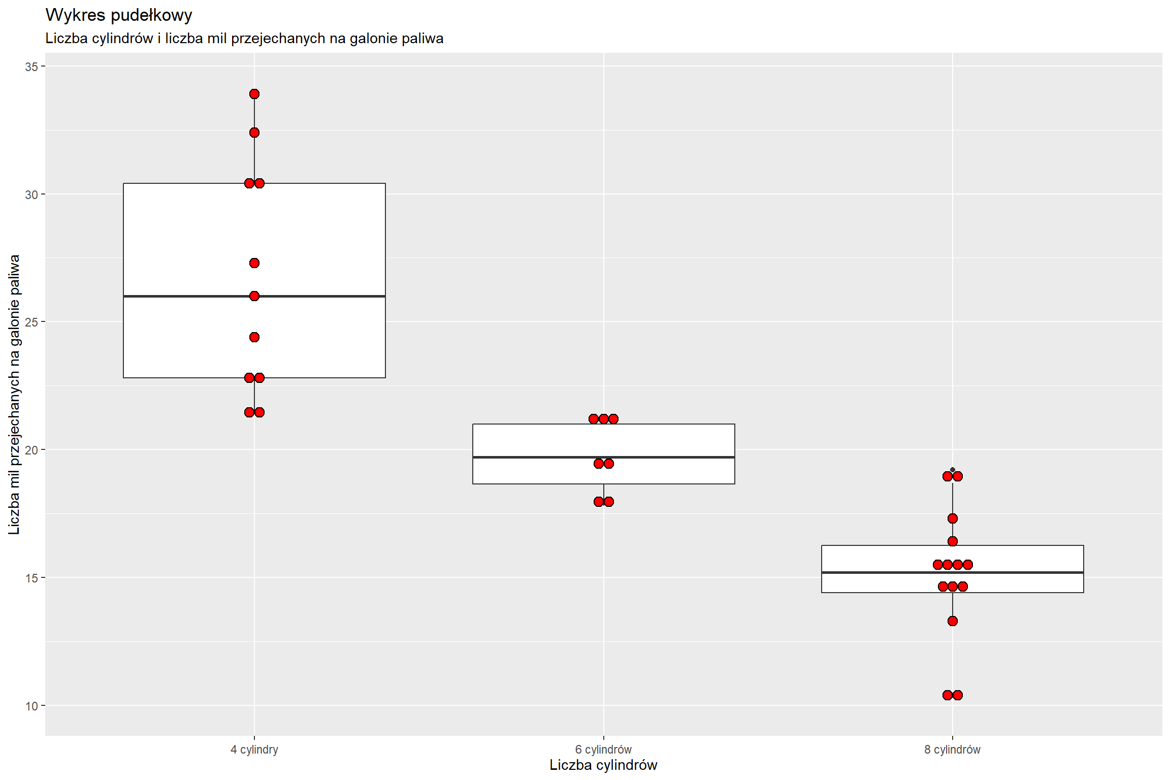
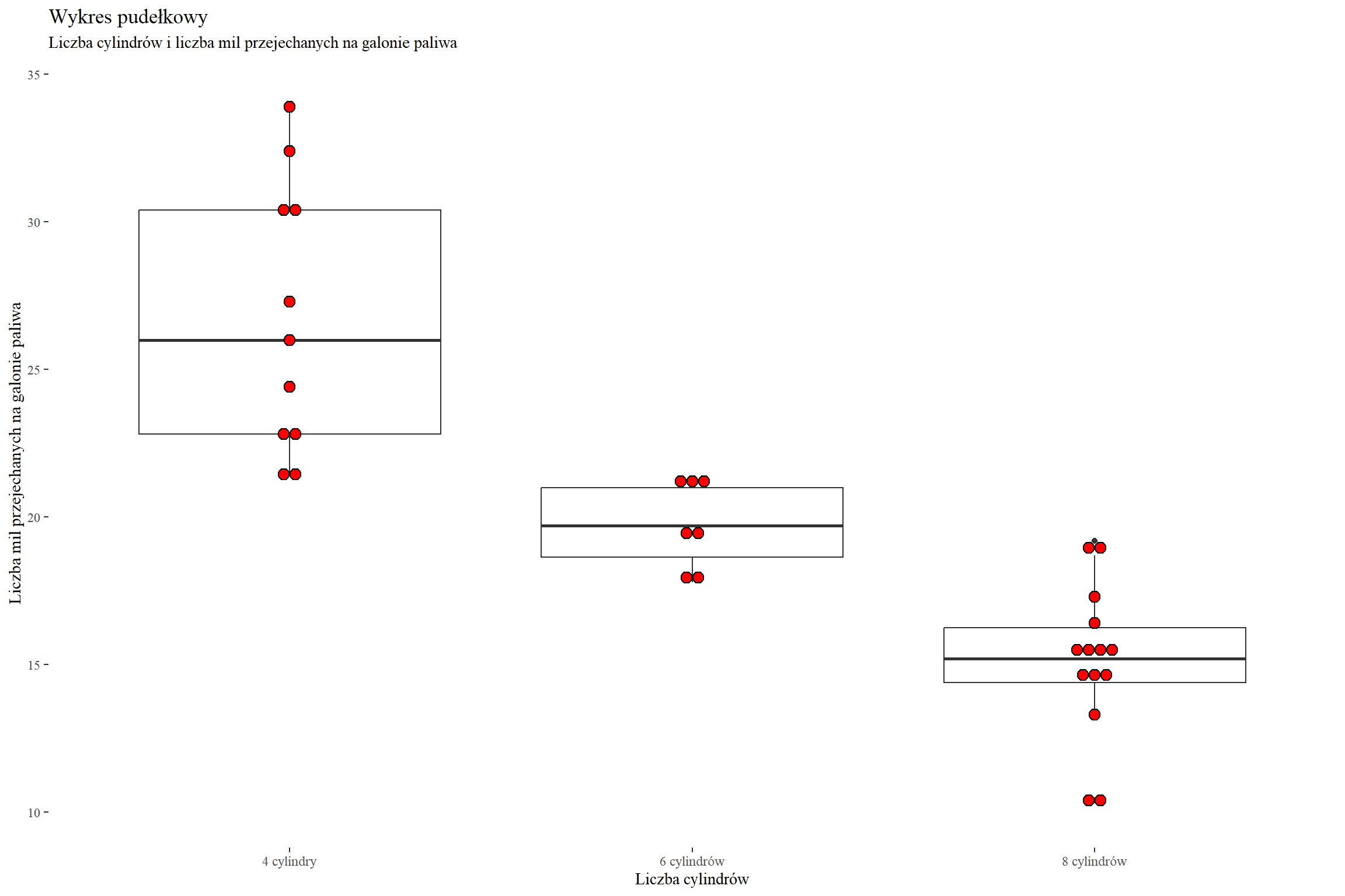
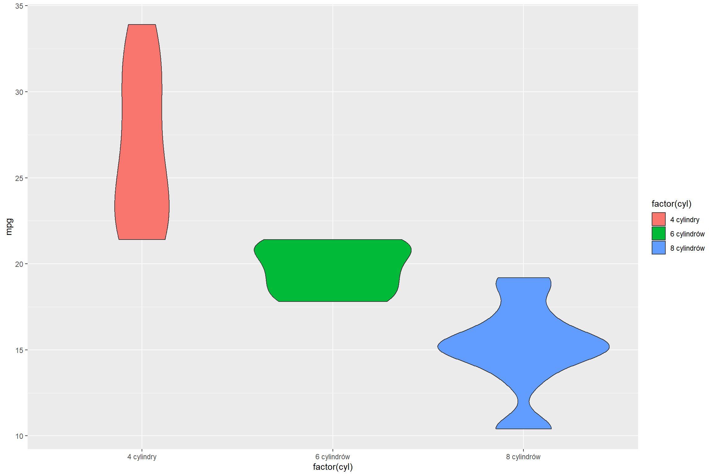
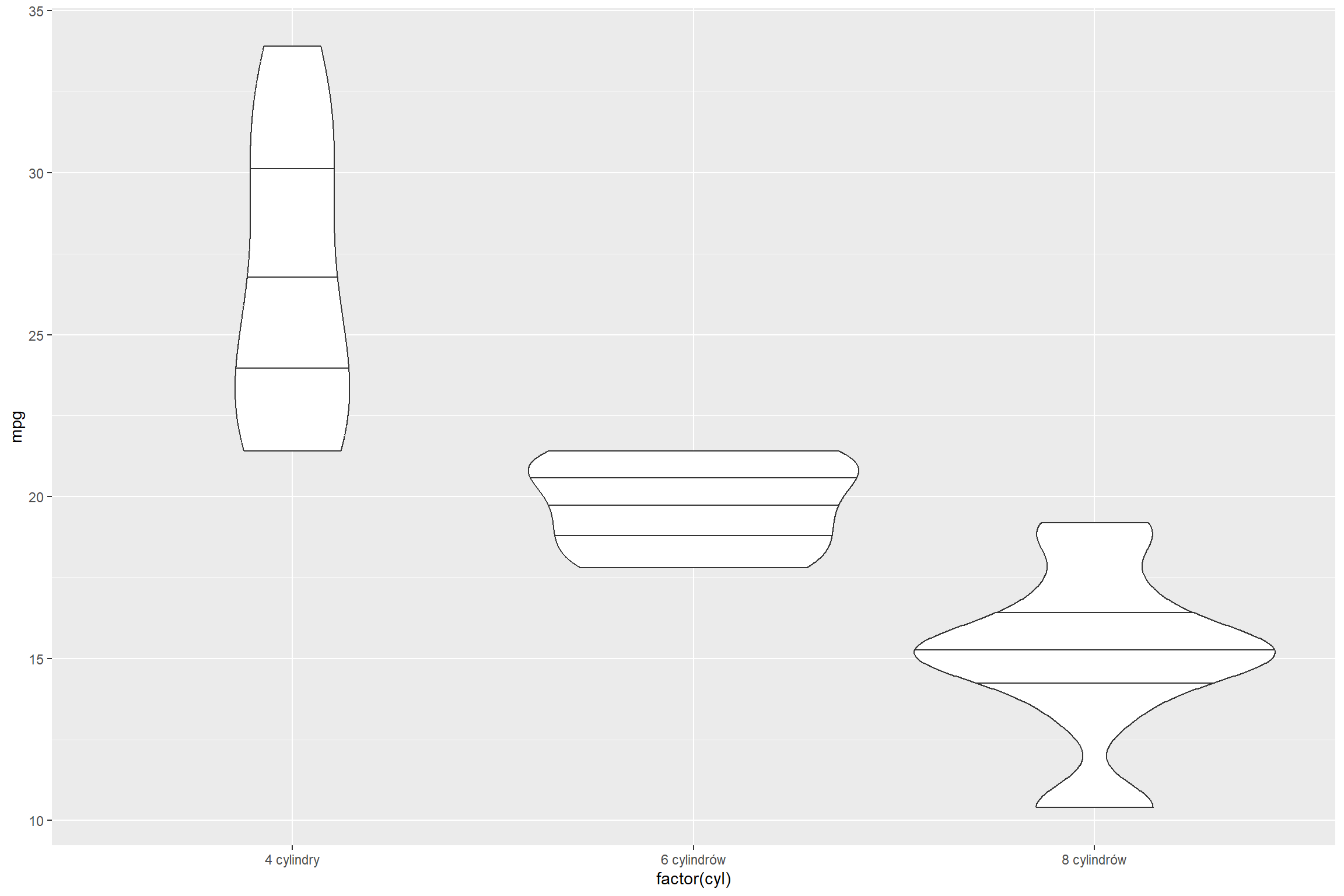
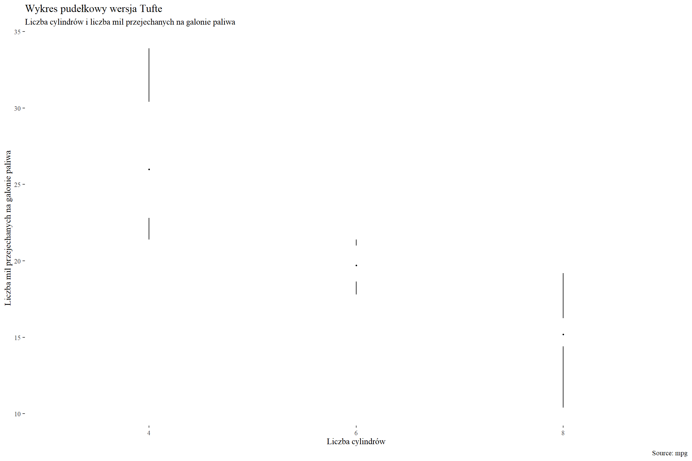
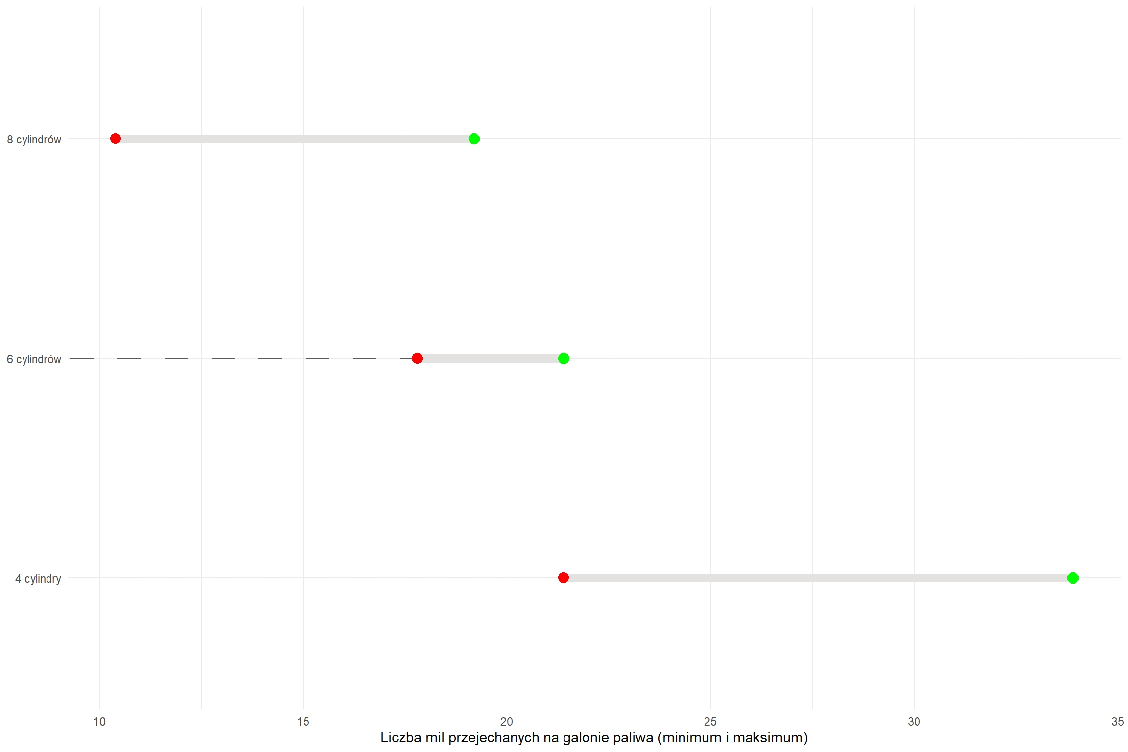
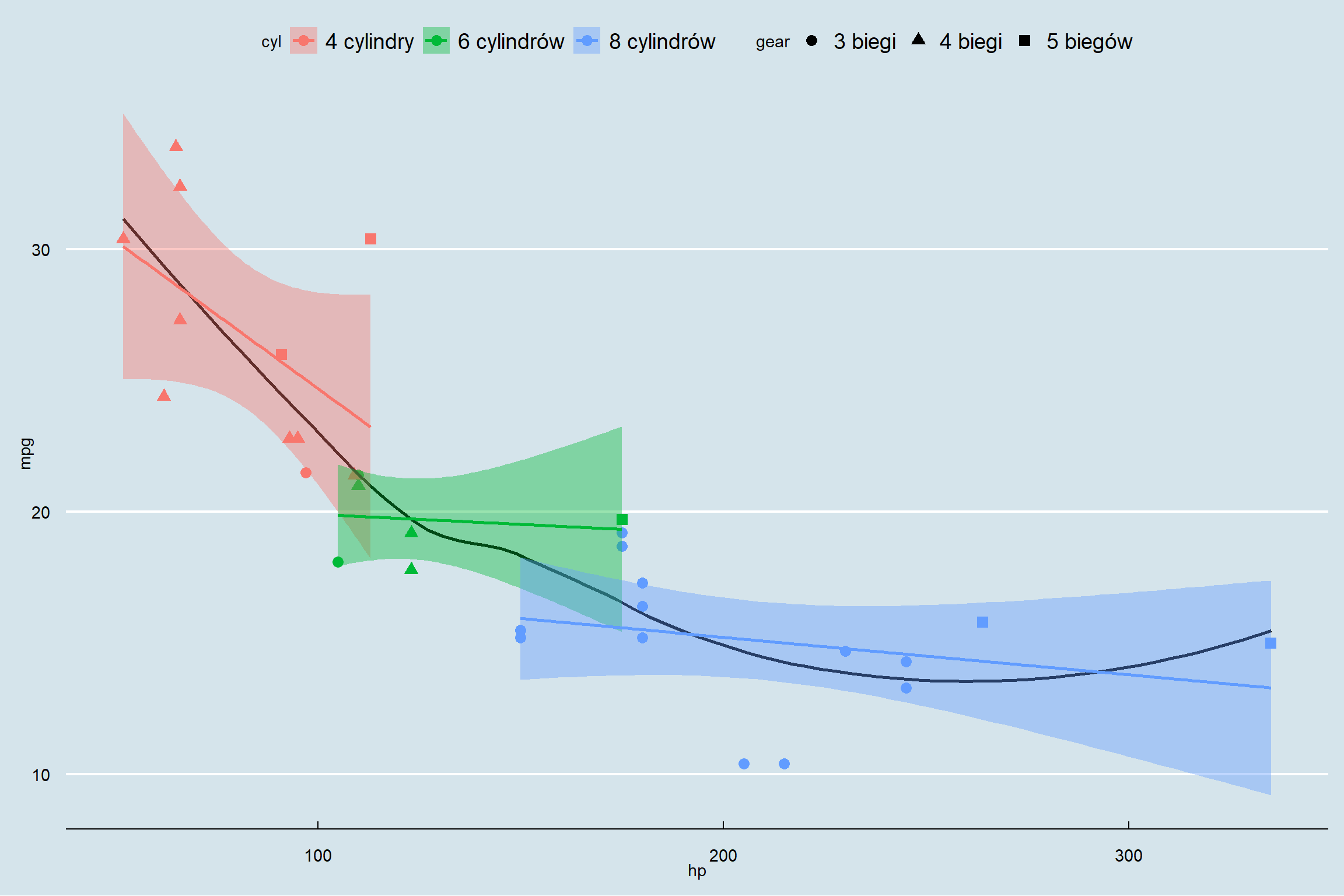
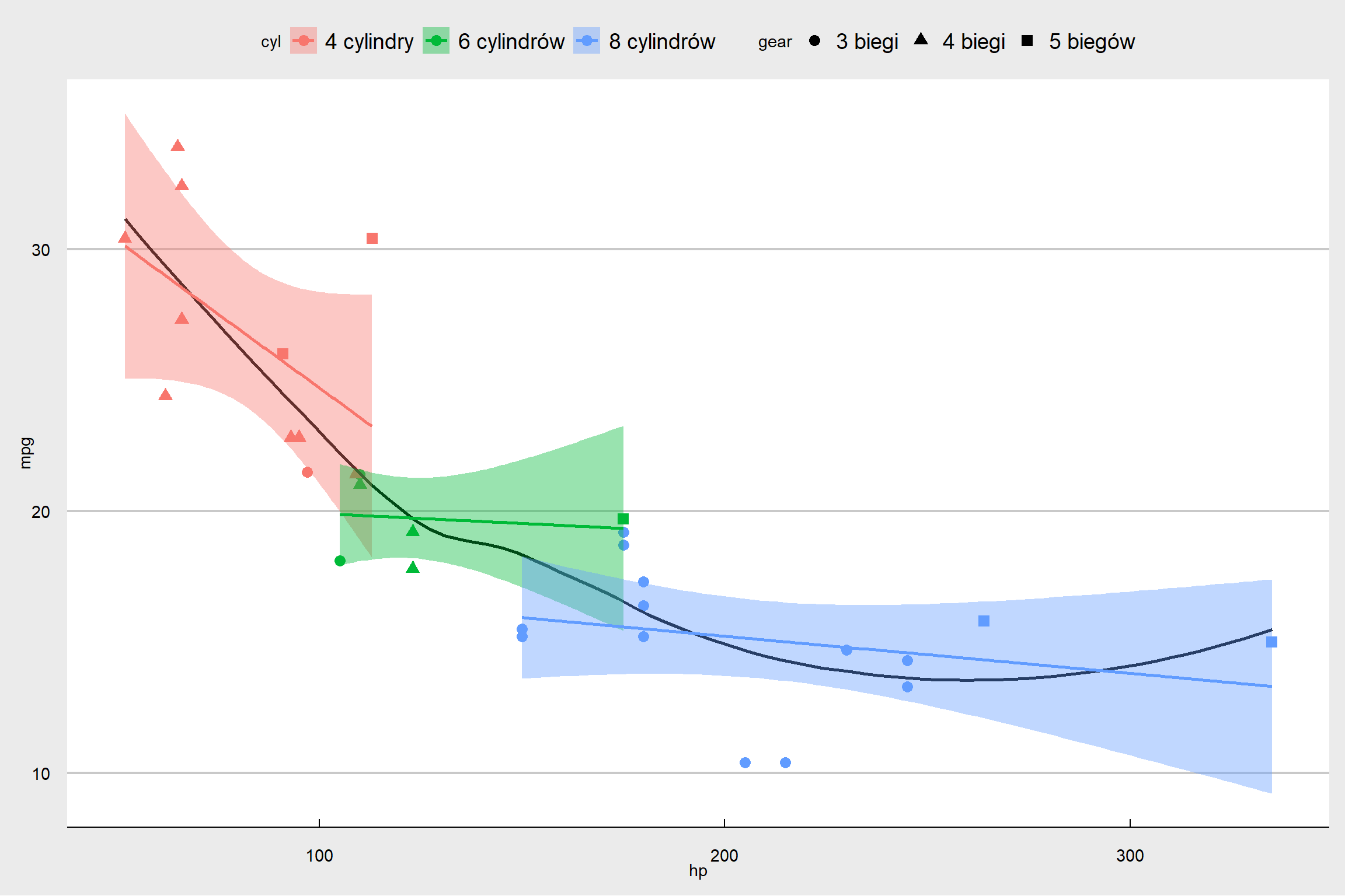
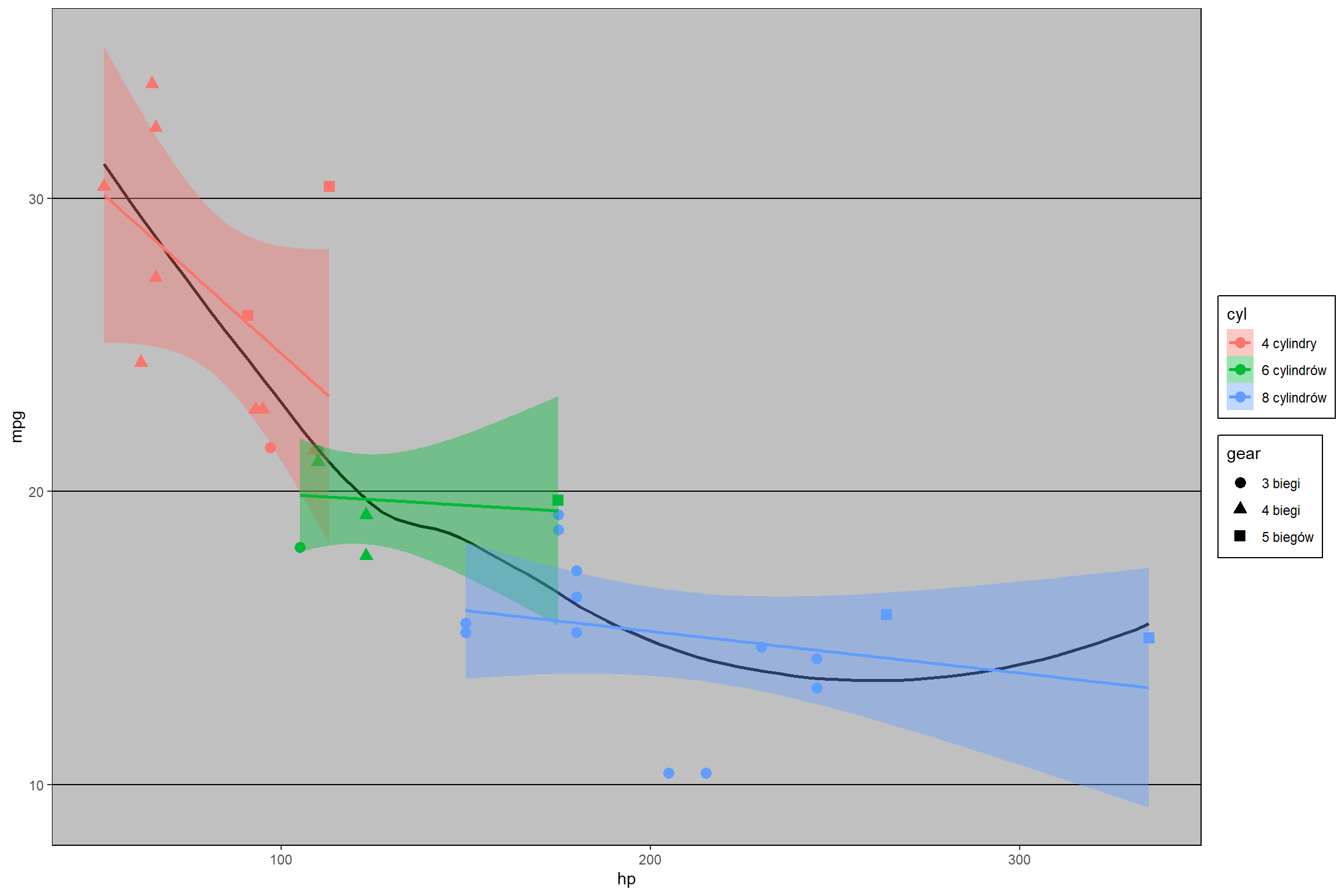
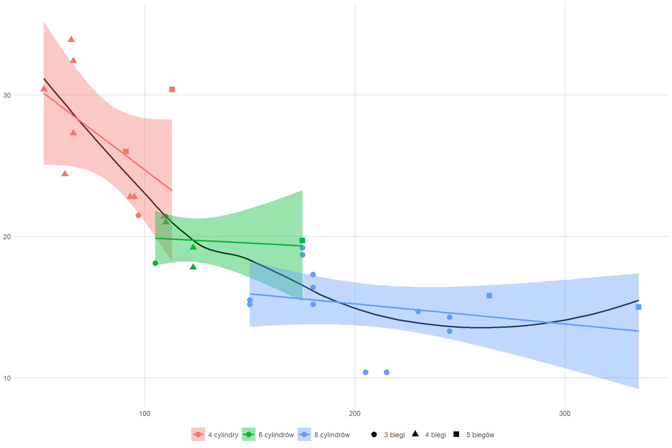
mtcars$cyl <- factor(mtcars$cyl,levels=c(4,6,8),labels=c('4 cylindry', '6 cylindrów', '8 cylindrów'))